June 2025
Quantum software today is split in two. Software stacks for digital quantum computers (gate-based) speak the language of quantum circuits. Analog stacks speak the language of Hamiltonians and time evolution, which is the native model for the analog quantum computers we build at Qilimanjaro. Most quantum computing companies choose between digital or analog to develop their own stack.
QiliSDK 0.2.0 does not. It is an open-source Python framework that unifies both paradigms behind a single, backend-agnostic API. The same program runs on CPU, GPU, or Quantum Processing Unit (QPU) by changing one line of code.
Check the full release note here.
What's inside
QiliSDK is built around three layers:
- Primitives. Gate, Circuit, and pre-built Ansatz classes for digital workflows. Hamiltonian and Schedule classes for analog workflows. A QTensor core type, a parameter / variable system, and a Model abstraction that linearises generic optimisation problems into QUBO form.
- Functionals. A unified abstraction for any quantum workflow (sampling a circuit, evolving a Hamiltonian, running a variational program) that any backend can execute through a common backend.execute(functional) interface.
- Backends. CPU (QiliSim and QuTiP), GPU (NVIDIA CUDA-Q wrapper), and digital and analog QPUs (SpeQtrum Cloud and On-Premise).
What's new in 0.2.0
QiliSim, a native C++ emulator Our default backend now runs in C++ with a Python interface. It supports quantum circuits, Hamiltonian time evolution and quantum reservoirs. All methods integrated with several emulation strategies can be selected through configuration objects, so the same program can be re-run with different numerical methods by editing one line.
Unified noise modelling. A NoiseModel can be defined once and applied across QiliSim and the CUDA backend. It covers state noise, control-parameter perturbations and readout noise. Each channel implements both Kraus and Lindblad representations, so the same model runs unchanged on digital or analog backends.
Quantum Reservoir Computing. New primitives (QuantumReservoir, ReservoirLayer, ReservoirInput) for Quantum AI workflows suited for near-term analog hardware.
QTensor in C++. The core quantum-tensor type is now native code. State preparation, observables, partial traces, entropy, fidelity calculations and tensor products all run faster. The API works as a standalone quantum-information toolkit.
OpenQASM 2/3 and QIR interoperability. Native import and export to OpenQASM 3, plus round-trip support for Microsoft’s QIR via pyqir. Installed as optional extras.
Trotterisation of analog evolution. A new TrotterizedSchedule ansatz compiles an analog Schedule into a parameterised digital circuit over a chosen number of Trotter steps. New convenience constructors: Schedule.linear(), .quadratic(), .polynomial(), .sinusoidal().
Spanish and Catalan docs. A new Tutorials section in the documentation, with translations into Spanish (ES) and Catalan (CA) alongside English.
Smaller improvements: composable CircuitTranspiler pipeline (gate fusion, identity-pair cancellation, multi-controlled-gate decomposition, SABRE-based routing); unified FunctionalResult and a Readout builder; CUDA 13 support; automatic QUBO linearisation of higher-order terms via Rosenberg penalties.
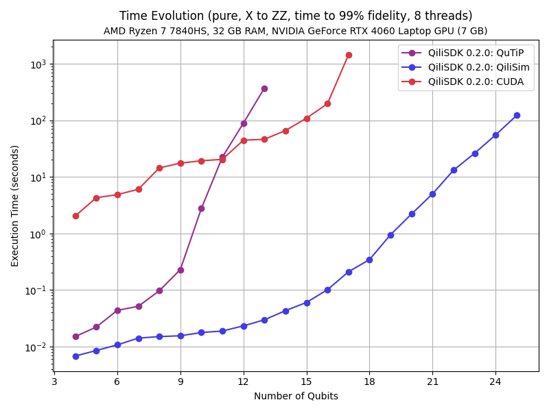
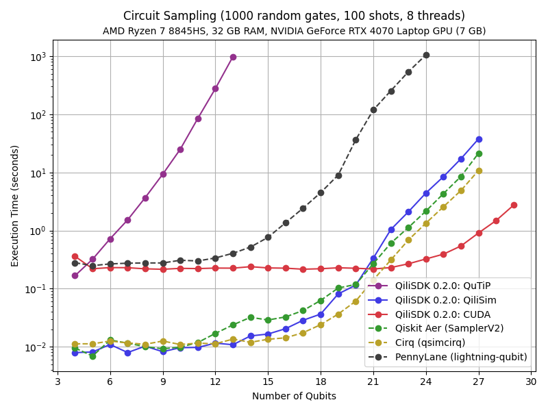
Performance
Two benchmarks ship with the release. On an analog annealing schedule reaching 99% fidelity with the exact ground state, QiliSim outperforms QuTiP and CUDA across the range tested, demonstrating efficient analog simulation on commodity CPU hardware.
On a digital workload (1.000 random gates, 100 shots), QiliSim is competitive with Qiskit Aer and Cirq for small to medium sizes, while the CUDA backend wins decisively at larger circuit sizes.
Get started
- Install: pip install qilisdk
- Docs (EN / ES / CA): https://qilimanjaro-tech.github.io/qilisdk/
- Source: https://github.com/qilimanjaro-tech/qilisdk
- Release notes: https://github.com/qilimanjaro-tech/qilisdk/releases/tag/0.2.0
- Cite: DOI 10.5281/zenodo.20411054