May 2026 – Qilimanjaro
Simulating the dynamics of quantum systems is one of the most promising near-term applications of quantum computing. It is also one of the hardest tasks for classical computers, which makes it a natural target for quantum advantage. Two main approaches compete for this goal: analog and digital quantum computing. They aim at the same dynamics through very different routes, and the cost of each route turns out to be very different too. In a recent whitepaper, we compared the two paradigms on a simple, representative bench-mark: the time evolution of the transverse-field Ising model on a two-dimensional lattice. The results are striking:
- No currently available digital quantum computer can reproduce the dynamics with the same precision (within a 5% error budget) that an analog device achieves directly.
- Even assuming fault-tolerant digital quantum computers exist, analog quantum computers are roughly ∼ 630× faster and consume around ∼ 90× less energy on the same task.
- Reaching the target precision digitally would require two-qubit gate fidelities three to six orders of magnitude beyond current state-of-the-art hardware.
In what follows, we unpack what these numbers mean and why they hold. For more information, check our whitepaper.
1. Two ways to simulate a quantum system
A quantum simulation answers a simple physics question: how does this system change over time? The two paradigms answer it in fundamentally different ways.
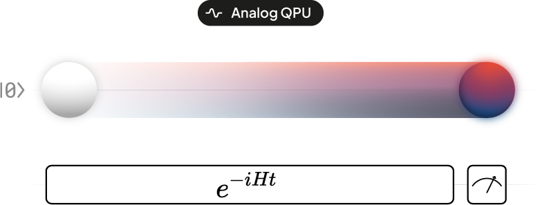
Analog quantum computers answer it directly. They build a physical system whose natural interactions match those of the problem of interest, switch it on, and let nature do the rest. The computer is the physics, so it does not need to translate the problem into anything else.
Digital quantum computers answer it indirectly. They approximate the same dynamics through a long sequence of discrete operations (quantum gates), much like a numerical integrator approximating a continuous function on a classical computer. They are universal, but they pay for that universality in circuit depth.
This split has been the central architectural debate in quantum computing for over a decade. Our work makes the trade-off quantitative for a concrete task.

2. The benchmark
We focus on a paradigmatic model in quantum many-body physics: the transverse-field Ising model. Spins sit on the vertices of a lattice, neighbouring spins interact, and an external field acts on each spin individually. We evolve this system for one microsecond on three lattice geometries that match Qilimanjaro’s hardware generations:

The target precision is a 5% total error budget. The question is then straightforward: how much does it cost – in time, gates, fidelity, and energy – to hit that target in each paradigm?
3. Trotterization: how digital simulation actually works
When a digital computer cannot apply the full Hamiltonian at once (because the different parts of the Hamiltonian do not commute), it breaks the evolution into many small steps. This is called Trotterization. The idea is simple: chop the total evolution time into δt small intervals, and within each interval apply the different parts of the Hamiltonian one after the other.
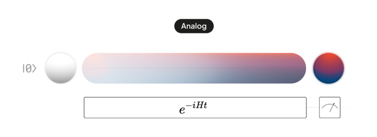
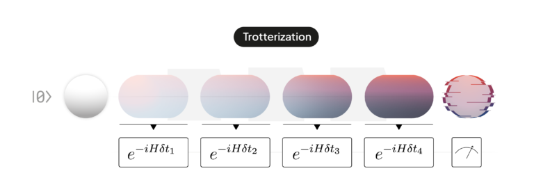
Figure 1: An analog continuous evolution (left) Trotterisation discretises a continuous evolution (right). Each step introduces a small approximation error, which decreases as the number of steps grows.
Smaller steps mean a more accurate approximation, but also more gates, and on a real, noisy device, more gates means more accumulated hardware error. So there is a sweet spot between “too few steps, too much approximation error” and “too many steps, too much hardware error”.
To improve on this trade-off, one can use higher-order Trotter formulas (called S2, S4, S6, and so on). They reduce the approximation error per step by combining several sub-steps in clever symmetric arrangements, making each step more accurate at the cost of being more expensive in gates. As we will see, higher order is not always better.
4. Today’s digital quantum computers cannot run these circuits
The first finding from the analysis is that none of the Trotter circuits required to reach 5% precision on the 5×5 lattice fit within the coherence time of current superconducting qubits, the window during which a qubit retains its quantum state. We take superconducting qubits as our reference because they are the fastest digital platform available today in terms of gate operation times. On slower platforms such as trapped ions, where two-qubit gates can be orders of magnitude slower, the circuit runtimes would be correspondingly longer and the gap to coherence times even wider.
Table 1: Circuit runtime versus typical multi-qubit coherence time (T2 ∼ 100 μs) for the 5×5 lattice.

Even the most compact decomposition (fourth-order Trotter) needs roughly six times longer than the qubits stay coherent. The first-order decomposition needs more than a thousand times longer. By the time the circuit finishes, the quantum information has long since decohered into noise.
Equivalently, hitting the target precision would require two-qubit gate error rates between 10−10 and 10−7, while today’s best superconducting hardware sits at around 10−3. Closing that gap requires quantum error correction, the fault-tolerant regime.
5. Even fault-tolerant digital simulation pays a energy bill
The natural counter-argument is: “fine, today digital can’t do it, but once fault tolerance arrives, the gap will close”. Our analysis suggests otherwise. Even assuming fault-tolerant digital quantum computers are available (and ignoring the substantial qubit overhead that fault tolerance itself demands), the runtime and energy gap persists.
The reason is structural. Both paradigms run inside a dilution refrigerator that draws around 19 kW continuously. The cooling infrastructure dominates the energy budget. What differs between paradigms is how long the cryostat needs to run to complete the computation:
Table 2: Energy per full experiment (5×5 lattice, 20 000 shots, 5% total error budget). The cryogenic baseline is the same for both paradigms; only the runtime changes.

Translated into operational cost at the US average retail electricity price (2025):

For a single experiment, fourth-order Trotter is still affordable. But quantum experiments are rarely run once: a typical parameter sweep involves hundreds or thousands of independent runs, so the analog advantage compounds quickly. And it grows with system size:
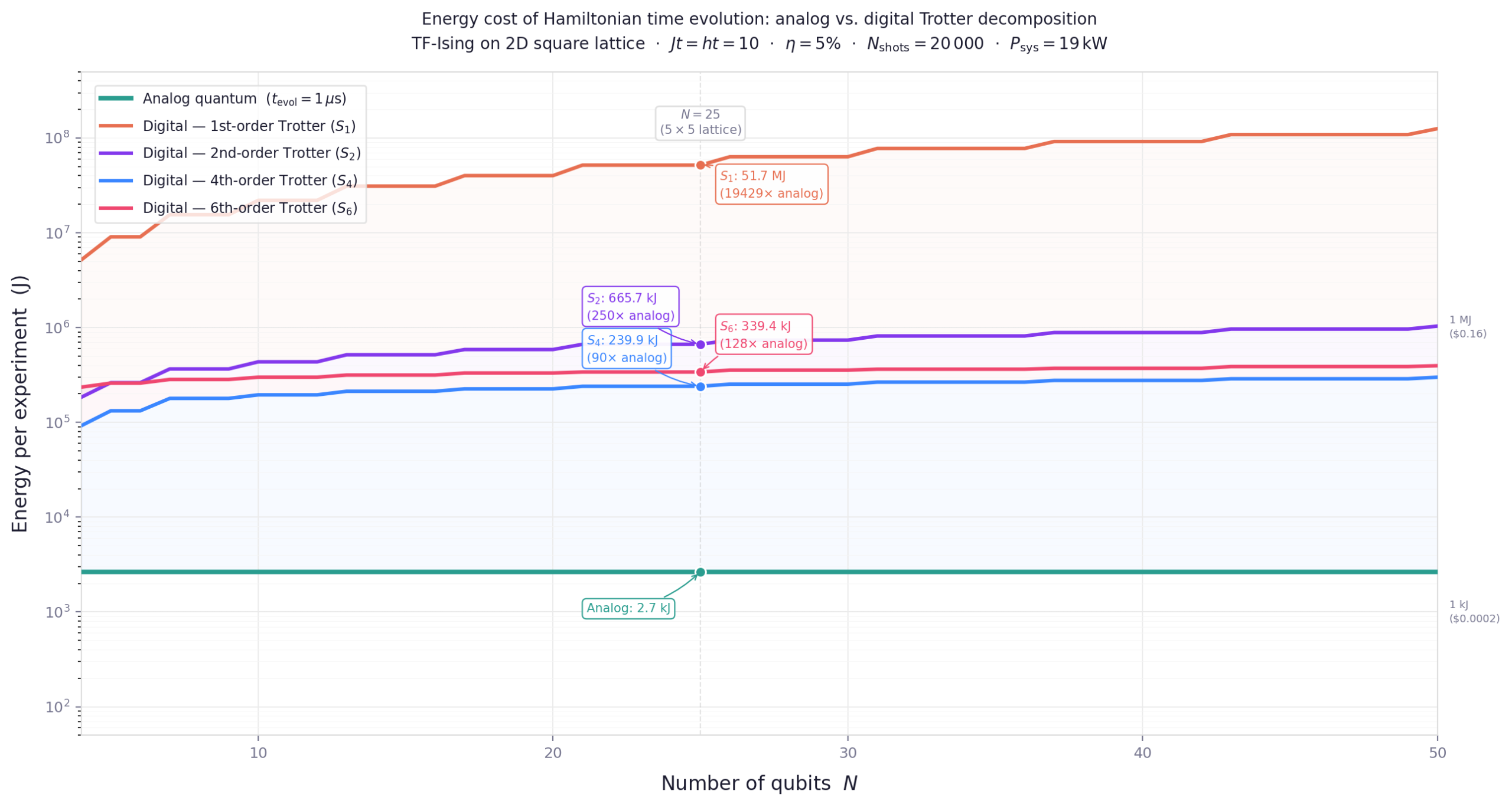
Figure 2: Energy cost per experiment as a function of system size N. The analog cost (horizontal line) is independent of N. Digital costs grow polynomially as N (1/p) for pth-order Trotter. The analog advantage widens with size for all orders.
Going to ever-higher Trotter orders does not keep improving the result. Going from first to second order reduces the runtime by a factor of ∼ 78. From second to fourth it gives another ∼2.8x improvement. But sixth order is worse than fourth: the circuit takes longer and consumes more energy.
The reason is that the number of gates per Trotter step grows roughly as 5(p/2) with the order p, while the number of steps required shrinks only polynomially. There is a finite optimal order, beyond which adding more “precision per step” costs more than it saves. For this benchmark, fourth-order Trotter is the sweet spot and going beyond it, decreases the precision of the calculation.
6. Implications
Our findings state that, digital quantum simulation of Hamiltonian dynamics, at the precision required for useful results, is neither achievable on present hardware nor competitive on future fault-tolerant hardware. The first claim follows from coherence times and gate fidelities that sit three to six orders of magnitude away from where they would need to be. The second follows from the structure of product-formula simulation itself: it approximates a continuous physical process through a discrete sequence of operations, and pays a runtime and energy overhead, roughly 90x respectively in our benchmark, that does not vanish in the fault-tolerant regime.
This gap is structural, not transient. It cannot be closed by better compilers or incremental hardware improvements, because it follows from the act of discretising the dynamics in the first place. An analog quantum computer runs the physics; a digital quantum computer approximates it.
For the broad class of problems centred on Hamiltonian dynamics, many-body quantum simulation, adiabatic quantum computation, quantum annealing, and quantum reservoir computing, analog quantum computers are the more resource-efficient platform today, and will remain so even as digital fault tolerance matures.